The number of registers in a Graphics Processing Unit (GPU) has been continuously grown over the last decade. A driving force of such growth is that although the number of cores has to be increased for better performance, the number of registers per core has to be maintained to provide sufficient thread parallelism for hiding memory latency, which is generally considered as challenging even with better process technology in a near future. Another aspect is that as GPUs are covering broader areas from graphics to artificial intelligence, applications will perform more complex work in a thread, thus will likely demand more registers.
For GPU registers, the data should be resident on chip as possible to enable fast context switching of threads as well as to feed massively parallel execution units. As a result, GPU register files consume substantial energy as well as on-chip storage. For instance, an NVIDIA GV100 GPU has a 256 KB register file per Streaming Multiprocessor (SM) and there are 80 SMs in the GPU, which corresponds to 20MB of registers [1]. According to previous studies, the register file consumes about 15 percent of SM energy [2]. Deep learning workloads, which are widely used in recent GPUs, also show similar energy consumption tendencies [3]. The energy consumption of register files for various deep learning algorithms is between 15 and 20 percent of SM energy.
A recent idea to improve both the energy and storage efficiency of the GPU register file is to compress register data [4,5]. There are unique aspects of GPUs that make register compression as a feasible option beyond widely adopted memory traffic compression [1,6]. A typical GPU executes a group of 32 threads on a vector execution unit. The grouped threads are collectively called a warp. In the vector unit, each scalar lane runs a thread. A vector register used in the vector unit is called a warp register. Previous studies have observed that the thread registers in a warp register have a strong similarity in values with each other [5,7]. Because of this value similarity, simple but efficient data compression algorithms such as base-delta-immediate (BDI) [3] are expected to be quite effective for compressing a warp register as a whole. Furthermore, GPUs' great latency tolerance enables them to allow additional compression stages in register access path while minimizing performance overheads due to increased pipeline depth. Compressed registers consume less energy for data transfer, and also require fewer bits to be stored in the register file which provides power gating opportunities for register banks.
Although previous studies have been explored register compression to some degree, a limit study is required to investigate its potential gain, given that the compression ratio varies significantly according to the choice of algorithm. As an indicator to guide how efficient a register compression algorithm is, this paper proposes an analytical model to calculate the ideal compression ratio which is known to be mathematical upper bound according to entropy theory. Our evaluation shows the theoretical maximum compression ratio can be obtained by 3.99, which is 2.33 times more than a previously proposed BDI based register compression algorithm [3].

 Previous papers have proposed several data compression techniques. Cache or memory system have been known to be good locations to compress data for many reasons, such as energy reduction [8], throughput improvement [9], or better cache or memory efficiency [10]. There are papers to leverage compression for improving efficiency or performance in the context of GPUs. For instance, Pekhimenko et al. proposed a toggle-aware compression to improve the memory bandwidth efficiency in GPUs [11]. Lal et al. utilized the Huffman coding for the GPU memory compression [12].
Lee $\textit{et al.}$ [5] proposed to compress the register data for GPU energy efficiency improvement. The proposed com-pression uses a variant of base-delta-immediate (BDI) compression, which was originally designed for cache compression [13]. GPU register compression is motivated by similarity between threads within a warp, which lead to an observation that BDI-like algorithms are well suited to exploit value similarity across thread lanes. Compressing registers can be leveraged to reduce power or to improve energy efficiency by reducing the number of register banks to store or access a warp register, thus saves dynamic energy for register fetching as well as static energy when combined with power gating unused register banks.
There have also been studies using STT-MRAM to improve energy efficiency. Li $\textit{et al.}$ [14] proposed a STT-MRAM register file architecture with SRAM buffer. Won $\textit{et al.}$ [15] proposed the STT-MRAM register file with SRAM in the form of a cache. GPU register file implementation using STT-MRAM can be used with other data compression techniques and allows for further energy efficiency improvements.

1. Lossless Compression

  According to Shannon`s source coding theorem [16], the compression ratio of lossless data compression is closely related to the entropy value of data which can be derived from how likely each source symbol to appear. The theorem basically says for a vector consists of N elements where each element is from the source symbol set E, if the distribution of occurrence of source symbols in the vector is independent and identically distributed random and the entropy of the information the vector has is $H(X)$ bits, then the lower bound of the data size when the vector is lossless compressed is $N$ $H(X)$ bits as $N \to \infty$.

  Fig. 1 is an example to illustrate how this principle can be applied to obtain an ideal compression ratio for register accesses. The first row shows an access stream consists of seven 2-bit thread register accesses. Thus 14 bits are needed to store the entire trace without compression. The second row shows only 13 bits are needed to store when the trace is compressed, with a hypothetical algorithm which maps from the source symbol $E \in \{0$, $1$, $2$, $3\}$ to the code word $c(X) = \{$``0'': 110, ``1'': 0, ``2'': 10, ``3'': 111$\}$. The lower bound of a code word based compression can be obtained from the results of entropy theory. Assuming the entropy $H(X)$ is given as a prior knowledge, the upper bound of the compression ratio, $C(X)$, can be derived from $E$ and $H(X)$ as follows:

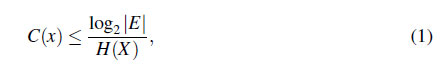
  where $\left| E \right|$ represents the number of elements in the set $E$. The last row shows how to calculate the lower bound of the code word length is 12.897 bits from the given $H(X)$ as shown in Fig. 1, which corresponds to the compression ratio of 1.086.

2. Entropy Model

  The key of our model is how to obtain $H(X)$ for register values. We first need assumptions about the compression granularity. The choice in this paper is to view each thread register value as a symbol. The insight under this decision is that there is structural value similarity between thread registers within a warp register [5], thus our selection can capture such similarity as well as benefits with optimal entropy coding. Further, we assume each thread register is 32-bit wide which is quite a common choice as most GPUs are optimized for 32-bit operations. Regardless of our choices, we believe the presented methodology is general enough to work with any other parameters.
Assume that $E$ is the set of all possible register values, thus $E=\{0$, $1$, $2$, $\dots$, $2^{32}-1 \}$ for a 32-bit wide register. We also define the sample space $\Omega$, which is a trace of register values observed during program execution. $\Omega$ can be constructed by collecting the register values written back to the register file while running applications on a simulator.
A discrete random variable for a register value observation event $X$ can be defined as $X :$ $\Omega \to E$. Since the register values are discrete by nature, we can define the probability mass function (PMF) $f_X(x)$ of $X$ which is defined as

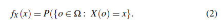
  $f_X(x)$ can be obtained by counting the number of occurrences for each register value $e \in E$ in $\Omega$. To derive $H(X)$, the information content $I(x)$ which is defined as the following:

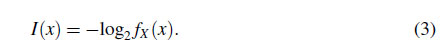
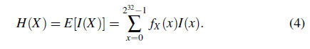
  $I(x)$ means the amount of information in bits when a particular register value $x$ is observed. Finally, the entropy $H(X)$ can be calculated from $I(x)$ as follows.

3. Optimizing for Application and Data Types

  Eqs. (1) and (4) imply that the ideal compression efficiency is determined from $f_X(x)$, and as the distribution of $f_X(x)$ is closer to uniform distribution the maximum achievable compression ratio $C(X)$ will approach to 1.0 as the entropy $H(X)$ will increase. At extreme, if $f_X(x)$ is a discrete uniform distribution, all register values will occur equally likely. In this case, the entropy is calculated as the following:

  $I(x)$ means the amount of information in bits when a particular register value $x$ is observed. Finally, the entropy $H(X)$ can be calculated from $I(x)$ as follows.

  In this case, the ideal compression ratio is $32/17.047 = 1.87$. Because entropy $H(X)$ varies according to $f_X(x)$, then it is needed to use different $f_X(x)$ for each application to better model ideal performance, as $f_X(x)$ will vary according to application characteristics. Our model uses different $f_X(x)$ for each application by collecting register access trace separately for each benchmark.
In similar reasons, our model can be further improved by accounting for data types, which leverages the fact that $f_X(x)$ also varies according to registers' data types. Fig. 2 shows the portion of register values for each of the four different data types: Signed integer (S32), unsigned integer (U32), floating point (F32), and untyped bit (B32). Registers with different data types will have different value patterns, thus optimizing the compression algorithm for each data type will likely lead to a higher compression ratio. Also, this result shows the most frequent data type is different in each of the applications, which further supports the argument that the optimal algorithm has to consider $f_X(x)\ $variation across applications.

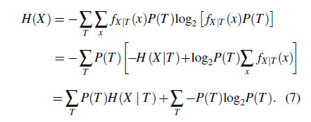
  Our model uses four conditional entropy values for the four data types, $H(X\mid S)$, $H(X\mid U)$, $H(X\mid F)$, and $H(X\mid B)$, where $T \in \{ S$, $U$, $F$, $B \}$. Each element in T means S32, U32, F32, and B32, respectively. The aggregated entropy $H(X)$ can be derived from the conditional entropy values and the portion of register accesses to each data type. The derivation is as follows:

4. Latency Model

  The program characteristic can be classified to compute-bounded or memory-bounded by analyzing the average stalled cycle of SM [2]. Under the phase of compute-bounded workloads, the core's average stalled cycle decreases, since execution units of SM are fully utilized. In this section, capability of SM directly influences the overall performance. On the contrary, SM's average stalled cycle increases when GPU encounters memory-bounded phase of the application. Because of the latency of the memory access or preparing the data for computation, the pipeline should wait until the access or preparation is finished.
Fig. 3 shows the ratio of the average stalled cycle during the heartwall application which is in Rodinia benchmark suite [17]. As shown in the figure, the characteristic of the ratio of the average stalled can be divided into two types, highly stalled phase and nearly non-stalled phase. These two phases appear one after the other during the execution of the application. To classify the application's characteristics whether the compute-bounded or memory-bounded, we use measured values of the stalled cycle's ratio. When the average ratio of compute-intensity is larger than memory-intensity, we can classify this phase as compute-bounded phase.

  Register compression introduces additional latency while fetching values from registers in compute-bounded phase. On the other hand, memory work is the bottleneck of the memory-bounded phase. Therefore, the memory-bounded phase is not influenced by register compression. Equation 8 shows the relative performance of the GPU that Amdahl's law [18] is applied to compute-bounded phase and memory-bounded phase.

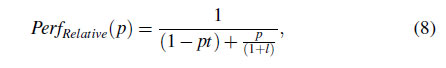
  where $p$ is the portion of compute-bounded phase ($0 \le p\le 1$) and $l$ is the additional latency of register compression.

1. Methodology

 We used 16 GPU applications selected from Rodinia [17], Parboil [19], and GPGPU-Sim [20] benchmark suites. We captured register access trace from GPGPU-Sim [20] and run a post-simulation on the data. The post simulation includes our compression model as well as an implementation of BDI-based register compression [5]. Our simulation approximates NVIDIA Fermi architecture [21] and Volta architecture [1] with the microarchitectural parameters listed in Table 1.

2. Entropy Values and Upper Bound of Compression Ratio

 Fig. 4 shows the entropy values of the 32-bit thread register values measured from 16 applications. $Y$-axis means the entropy value in bits. We first measured the entropy values for each of the four data types explained in Section III-1. The modeled upper bound number is derived from Equation and the collected per-type entropy values and $f_X(x)$ data. The entropy bits can be understood how many bits are required to store a register.

3. Compression Ratio with Existing Technique

 Fig. 6 compares compression ratio for the integer type registers of the evaluated applications. GPU microarchitectural parameters from BDI compression [5] were used. The bar labeled BDI shows the compression ratio when BDI compression algorithm is used for register file [5]. All benchmarks combined, the calculated ideal case compression ratio is $3.99\times$, which is significantly higher than $2.33\times$ of the compared BDI register compression. We noticed LIB is the most outstanding case where BDI efficiency is close to the ideal case. On a closer look of the actual register values, we observed the majority of register values are zero, which is the case where the BDI compression can achieve highest compression efficiency close to ideal. In most other applications, the efficiency of BDI appears to be from 21% to 57% compared with the upper bound from our ideal compression model. A hypothetical algorithm may be able to perform 29% to 623% better than the BDI compression, which implies headroom for further improvement.

4. Energy Efficiency

 Fig. 7 represents dynamic energy of individual hardware components of the LIB application from GPUWattch [2]. GPU microarchitectural parameters from NVIDIA Fermi architecture [21] were used. Dynamic energy was measured for each kernel within the application. The percentage of energy consumed by the register file with ideal compression ratio in the LIB application was measured to be 1.27% and 0.99%, respectively. Since the register file consumes about 15 percent of SM energy, the limit of energy efficiency improvement cannot exceed the energy consumed by the register file.

  This paper proposed an entropy-based compression model to study theoretical limits of GPU register compression algorithms. We provided a method to obtain the entropy function from empirically profiled register value traces. The model is then further refined to account for application and data type variations. Experimental results show that an existing algorithm is still underperforming compared with our model. A hypothetical algorithm may achieve higher compression ratio which would lead to more energy efficient GPUs.

  This work has been supported by Global Education and Research Center for Convergence Technology, a Brain Korea 21 four program, Yonsei University.